Implementing your own neural network can be hard, especially if you’re like me, coming from a computer science background, math equations/syntax makes you dizzy and you would understand things better using actual code.
Today I’ll show you how easy it is to implement a flexible neural network and train it using the backpropagation algorithm. I’ll be implementing this in Python using only NumPy as an external library.
After reading this post, you should understand the following:
- How to feed forward inputs to a neural network.
- Use the Backpropagation algorithm to train a neural network.
- Use the neural network to solve a problem.
In this post, we’ll use our neural network to solve a very simple problem: Binary AND.
The code source of the implementation is available here.
Background knowledge
In order to easily follow and understand this post, you’ll need to know the following:
- The basics of Python / OOP.
- An idea of calculus (e.g. dot products, derivatives).
- An idea of neural networks.
- (Optional) How to work with NumPy.
Rest assured though, I’ll try to explain everything I do/use here.
Neural networks
Before throwing ourselves into our favourite IDE, we must understand what exactly are neural networks (or more precisely, feedforward neural networks).
A feedforward neural network (also called a multilayer perceptron) is an artificial neural network where all its layers are connected but do not form a circle. Meaning that the network is not recurrent and there are no feedback connections.
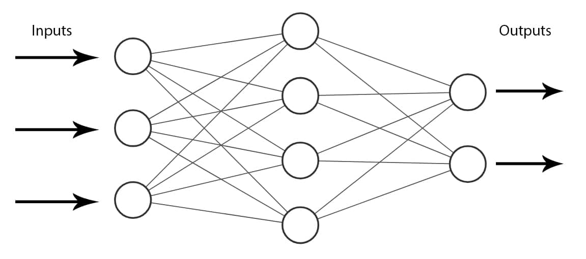
An example of a Feedforward Neural Network
These neural networks try and approximate a function $f(X)$ where $X$ are the inputs that get fed forward through the network to give us an output.
The lines connecting the network’s nodes (neurons) are called weights, typically numbers (floats) between 0 and 1.
Also, each neuron has a bias unit (a float between 0 and 1) that helps shift the results.
These are called the parameters of the network.
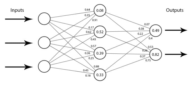
An example of a network's parameters
When inputs are fed forward through the network, each layer will calculate the dot product between its weights and the inputs, add its bias then activate the result using an activation function (e.g. sigmoid, tanh).
$$ (X\cdot W_l + \beta_l) $$
These activation functions are used to introduce non linearity.
Implementing a flexible neural network
In order for our implementation to be called flexible, we should be able to add/remove layers without changing the code. This means that hard-coding weights and layers is a no go.
First of all, let’s import NumPy and set a seed for us to get the same results when generating random numbers:
import numpy as np

np.random.seed(100)
Layers
We’ll create a class that represents our network’s hidden and output layers.
class Layer:
    """
    Represents a layer (hidden or output) in our neural network.
    """
Initialisation
def __init__(self, n_input, n_neurons, activation=None, weights=None, bias=None):
    """
    :param int n_input: The input size (coming from the input layer or a previous hidden layer)
    :param int n_neurons: The number of neurons in this layer.
    :param str activation: The activation function to use (if any).
    :param weights: The layer's weights.
    :param bias: The layer's bias.
    """

    self.weights = weights if weights is not None else np.random.rand(n_input, n_neurons)
    self.activation = activation
    self.bias = bias if bias is not None else np.random.rand(n_neurons)
In the class’s constructor __init__ we’ll initialize the layer’s weights and bias using the length of the input and the number of neurons this layer has. Specifying the weights and bias is optional as they will be randomly generated if not provided.
Note: The layer’s input is not always our initial input $X$, it can also be the output of a previous layer.
If we take the network shown in the figures above, we can represent its first hidden layer (3 x 4) as follows: hidden_layer_1 = Layer(3, 4).
As a result, the weights and bias will be:
Weights: [[0.54340494 0.27836939 0.42451759 0.84477613]
          [0.00471886 0.12156912  0.67074908 0.82585276]
          [0.13670659 0.57509333 0.89132195 0.20920212]]

Bias:   [0.18532822 0.10837689 0.21969749 0.97862378]
Printed out nicely, we get:
$$ W_l = \begin{bmatrix} 0.54 & 0.27 & 0.42 & 0.84 \newline 0.00 & 0.12 & 0.67 & 0.82 \newline 0.13 & 0.57 & 0.89 & 0.20 \end{bmatrix} , \beta_l = \begin{bmatrix} 0.18 \newline 0.10 \newline 0.21 \newline 0.97 \end{bmatrix} $$
The columns in the weights matrix $W_l$ represent our layer’s neurons and each row is the weights between one input neuron and all our layer’s neurons.
Activation
As the inputs get fed forward through our network, each layer must calculate the output using its weights and the received inputs, apply an activation function (if chosen) on the output then return the result to us.
def activate(self, x):
    """
    Calculates the dot product of this layer.
    :param x: The input.
    :return: The result.
    """

    r = np.dot(x, self.weights) + self.bias
    self.last_activation = self._apply_activation(r)
    return self.last_activation

def _apply_activation(self, r):
    """
    Applies the chosen activation function (if any).
    :param r: The normal value.
    :return: The activated value.
    """

    # In case no activation function was chosen
    if self.activation is None:
        return r

    # tanh
    if self.activation == 'tanh':
        return np.tanh(r)

    # sigmoid
    if self.activation == 'sigmoid':
        return 1 / (1 + np.exp(-r))

    return r
Here’s an explanation of the process:
- The input goes through our
activatefunction. - It calculates $X\cdot W_l + \beta_l$.
- Applies the chosen activation function $A(r)$.
- Saves the result in
last_activation(I’ll explain why later). - Returns the result.
Note: I only implemented here 2 activation functions, tanh $(2 \cdot \sigma \left( 2 x \right) - 1)$ and sigmoid $(\frac{1}{1 - e^{-x}})$, but there are many more available.
If we want to active the input [1, 2, 3] for example, we’ll write the following: layer.activate([1, 2, 3]), which results in: [1.14829064 2.35516451 4.65967912 4.10271179], a vector of length 4 (our number of neurons).
$$ r = \begin{bmatrix} 0.54 & 0.27 & 0.42 & 0.84 \newline 0.00 & 0.12 & 0.67 & 0.82 \newline 0.13 & 0.57 & 0.89 & 0.20 \end{bmatrix} \cdot \begin{bmatrix} 1 \newline 2 \newline 3 \end{bmatrix} + \begin{bmatrix} 0.18 \newline 0.10 \newline 0.21 \newline 0.97 \end{bmatrix} = \begin{bmatrix} 1.15 \newline 2.35 \newline 4.66 \newline 4.10 \end{bmatrix} $$
The dot product between a matrix $A(N\times M)$ and a vector $V(N)$ is simply a new vector $R(M)$ made of dot products between each element in $V$ and each row $A_i$. You can find more information about this here.
Don’t forget that we didn’t specify any activation function, so the result we’re seeing here is only the dot product.
If we did actually specify one, let’s say sigmoid, then the result would be the following (note that all the values are now between 0 and 1):
$$ \sigma( \begin{bmatrix} 1.15 \newline 2.35 \newline 4.66 \newline 4.10 \end{bmatrix} ) = \begin{bmatrix} 0.76 \newline 0.91 \newline 0.99 \newline 0.98 \end{bmatrix} $$
Neural network
We’ll also create a class to represent a neural network:
class NeuralNetwork:
    """
    Represents a neural network.
    """

    def __init__(self):
        self._layers = []

    def add_layer(self, layer):
        """
        Adds a layer to the neural network.
        :param Layer layer: The layer to add.
        """

        self._layers.append(layer)
The code is pretty straight forward, we have a constructor a initialize an empty list _layers and a function add_layer that appends layers to that list (of course, the layers are of type Layer, the one we created earlier).
Feed forward
As previously explained, inputs travel forward through the network.
We’ll go ahead and implement it in our NeuralNetwork class:
def feed_forward(self, X):
    """
    Feed forward the input through the layers.
    :param X: The input values.
    :return: The result.
    """

    for layer in self._layers:
        X = layer.activate(X)

    return X

"""
N.B: Having a sigmoid activation in the output layer can be interpreted
as expecting probabilities as outputs.
W'll need to choose a winning class, this is usually done by choosing the
index of the biggest probability.
"""
def predict(self, X):
    """
    Predicts a class (or classes).
    :param X: The input values.
    :return: The predictions.
    """

    ff = self.feed_forward(X)

    # One row
    if ff.ndim == 1:
        return np.argmax(ff)

    # Multiple rows
    return np.argmax(ff, axis=1)
- The function
feed_forwardtakes the input $X$ and feeds it forward through all our layers. - Each next layer will take the output of the previous one as the new input.
- The function
predictchooses the winning probability and returns its index (interpreted as the winning class).
Our neural network
Let’s now create a neural network that we will use throughout the post.
nn = NeuralNetwork()
nn.add_layer(Layer(2, 3, 'tanh'))
nn.add_layer(Layer(3, 3, 'sigmoid'))
nn.add_layer(Layer(3, 2, 'sigmoid'))
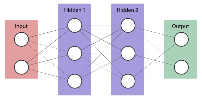
Representation of a neural network
Our neural network’s goal is to be able to perform the Binary AND operation.
Although at the moment, it sucks at it:
nn.predict([[0, 0], [0, 1], [1, 0], [1, 1]])
> [1 1 1 1]
| A | B | A ∧ B | Predicted |
|---|---|---|---|
| 0 | 0 | 0 | 1 |
| 0 | 1 | 0 | 1 |
| 1 | 0 | 0 | 1 |
| 1 | 1 | 1 | 1 |
Backpropagation
Now we’re at the most important step of our implementation, the backpropagation algorithm.
Simply put, the backpropagation is a method that calculates gradients which are then used to train neural networks by modifying their weights for better results/predictions.
The algorithm is supervised, meaning that we’ll need to provide examples (inputs and targets) of how it should work in order for it to actually help us.
In this implementation, we’ll use the Mean Squared Sum Loss as the loss function for the backpropagation algorithm, where $y_i$ is the target value and $^y_i$ is the predicted value. $$ \frac{1}{2}\sum{(y_i - ^y_i)}^2 $$
How does it work
Let’s represent our neural network the following way:
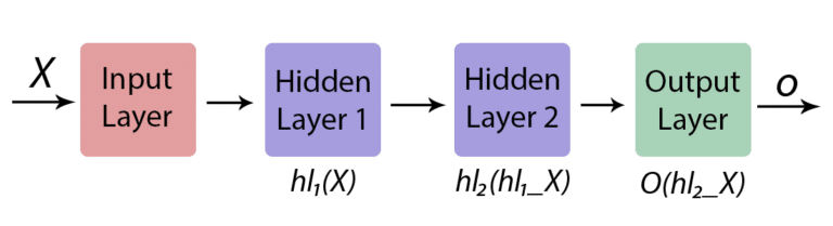
Simpler representation of our neural network
Where $hl_1X$ and $hl_2X$ are the outputs of the hidden layer 1 and the hidden layer 2. We can then see that the output is simply a chain of functions: $$ o = O(hl_2(hl_1(X)) $$
Calculating the gradients and changing our weights is now a step closer, all we have to do is use the Chain Rule and update every single weight we have.
If you want to read more about the exact math behind this, I highly recommend you this article.
Calculating the errors and the deltas
For each layer starting from the last layer (output layer):
- Calculate the error $E$:
For the output layer: $y - o$ where $o$ is the output that we get from
feed_forward(X). For the hidden layers: $W_{l+1} \cdot \delta_{l+1}$ where $l+1$ is the next layer and $\delta$ is its delta. - Calculate the delta: $E \times A'(o_i)$ where $A'$ is the derivative of our activation function and $o_i$ is the last activation that we stored previously.
First, let’s add the derivatives of our activation functions:
def apply_activation_derivative(self, r):
    """
    Applies the derivative of the activation function (if any).
    :param r: The normal value.
    :return: The "derived" value.
    """

    # We use 'r' directly here because its already activated, the only values that
    # are used in this function are the last activations that were saved.

    if self.activation is None:
        return r

    if self.activation == 'tanh':
        return 1 - r ** 2

    if self.activation == 'sigmoid':
        return r * (1 - r)

    return r
Then calculate the errors and the deltas:
def backpropagation(self, X, y, learning_rate):
    """
    Performs the backward propagation algorithm and updates the layers weights.
    :param X: The input values.
    :param y: The target values.
    :param float learning_rate: The learning rate (between 0 and 1).
    """

    # Feed forward for the output
    output = self.feed_forward(X)

    # Loop over the layers backward
    for i in reversed(range(len(self._layers))):
        layer = self._layers[i]

        # If this is the output layer
        if layer == self._layers[-1]:
            layer.error = y - output
            # The output = layer.last_activation in this case
            layer.delta = layer.error * layer.apply_activation_derivative(output)
        else:
            next_layer = self._layers[i + 1]
            layer.error = np.dot(next_layer.weights, next_layer.delta)
            layer.delta = layer.error * layer.apply_activation_derivative(layer.last_activation)
Updating the weights
All we have to do now is update our weight matrices using the calculated deltas and a learning rate.
The learning rate is a number between 0 and 1 that controls how much we adjust the weights. A big learning rate may cause you to miss the global minimum while a small learning rate might be too slow to converge.
for i in range(len(self._layers)):
    layer = self._layers[i]
    # The input is either the previous layers output or X itself (for the first hidden layer)
    input_to_use = np.atleast_2d(X if i == 0 else self._layers[i - 1].last_activation)
    layer.weights += layer.delta * input_to_use.T * learning_rate
- Loop over the layers (forwardly).
- Choose the input to use ($X$ or $o_{l-1}$) depending on the current layer.
- Update the layer’s weights using $W_l = W_l + \delta_l \times X^T \times \alpha$.
Our backpropagation function becomes:
def backpropagation(self, X, y, learning_rate):
    """
    Performs the backward propagation algorithm and updates the layers weights.
    :param X: The input values.
    :param y: The target values.
    :param float learning_rate: The learning rate (between 0 and 1).
    """

    # Feed forward for the output
    output = self.feed_forward(X)

    # Loop over the layers backward
    for i in reversed(range(len(self._layers))):
        layer = self._layers[i]

        # If this is the output layer
        if layer == self._layers[-1]:
            layer.error = y - output
            # The output = layer.last_activation in this case
            layer.delta = layer.error * layer.apply_activation_derivative(output)
        else:
            next_layer = self._layers[i + 1]
            layer.error = np.dot(next_layer.weights, next_layer.delta)
            layer.delta = layer.error * layer.apply_activation_derivative(layer.last_activation)

    # Update the weights
    for i in range(len(self._layers)):
        layer = self._layers[i]
        # The input is either the previous layers output or X itself (for the first hidden layer)
        input_to_use = np.atleast_2d(X if i == 0 else self._layers[i - 1].last_activation)
        layer.weights += layer.delta * input_to_use.T * learning_rate
Training the neural network
Finally, we need to train our neural network using the backpropagation function we implemented above.
We will use the stochastic gradient descent algorithm, where we update the weights with each row of our input (you can also take mini-batches instead).
def train(self, X, y, learning_rate, max_epochs):
    """
    Trains the neural network using backpropagation.
    :param X: The input values.
    :param y: The target values.
    :param float learning_rate: The learning rate (between 0 and 1).
    :param int max_epochs: The maximum number of epochs (cycles).
    :return: The list of calculated MSE errors.
    """

    mses = []

    for i in range(max_epochs):
        for j in range(len(X)):
            self.backpropagation(X[j], y[j], learning_rate)
        if i % 10 == 0:
            mse = np.mean(np.square(y - nn.feed_forward(X)))
            mses.append(mse)
            print('Epoch: #%s, MSE: %f' % (i, float(mse)))

    return mses
We repeat the process for max_epochs epochs (also called cycles or runs).
At every 10th epoch, we will print out the Mean Squared Error and save it in mses which we will return at the end.
Here’s the complete implementation:
import numpy as np

np.random.seed(100)


class Layer:
    """
    Represents a layer (hidden or output) in our neural network.
    """

    def __init__(self, n_input, n_neurons, activation=None, weights=None, bias=None):
        """
        :param int n_input: The input size (coming from the input layer or a previous hidden layer)
        :param int n_neurons: The number of neurons in this layer.
        :param str activation: The activation function to use (if any).
        :param weights: The layer's weights.
        :param bias: The layer's bias.
        """

        self.weights = weights if weights is not None else np.random.rand(n_input, n_neurons)
        self.activation = activation
        self.bias = bias if bias is not None else np.random.rand(n_neurons)
        self.last_activation = None
        self.error = None
        self.delta = None

    def activate(self, x):
        """
        Calculates the dot product of this layer.
        :param x: The input.
        :return: The result.
        """

        r = np.dot(x, self.weights) + self.bias
        self.last_activation = self._apply_activation(r)
        return self.last_activation

    def _apply_activation(self, r):
        """
        Applies the chosen activation function (if any).
        :param r: The normal value.
        :return: The "activated" value.
        """

        # In case no activation function was chosen
        if self.activation is None:
            return r

        # tanh
        if self.activation == 'tanh':
            return np.tanh(r)

        # sigmoid
        if self.activation == 'sigmoid':
            return 1 / (1 + np.exp(-r))

        return r

    def apply_activation_derivative(self, r):
        """
        Applies the derivative of the activation function (if any).
        :param r: The normal value.
        :return: The "derived" value.
        """

        # We use 'r' directly here because its already activated, the only values that
        # are used in this function are the last activations that were saved.

        if self.activation is None:
            return r

        if self.activation == 'tanh':
            return 1 - r ** 2

        if self.activation == 'sigmoid':
            return r * (1 - r)

        return r


class NeuralNetwork:
    """
    Represents a neural network.
    """

    def __init__(self):
        self._layers = []

    def add_layer(self, layer):
        """
        Adds a layer to the neural network.
        :param Layer layer: The layer to add.
        """

        self._layers.append(layer)

    def feed_forward(self, X):
        """
        Feed forward the input through the layers.
        :param X: The input values.
        :return: The result.
        """

        for layer in self._layers:
            X = layer.activate(X)

        return X

    def predict(self, X):
        """
        Predicts a class (or classes).
        :param X: The input values.
        :return: The predictions.
        """

        ff = self.feed_forward(X)

        # One row
        if ff.ndim == 1:
            return np.argmax(ff)

        # Multiple rows
        return np.argmax(ff, axis=1)

    def backpropagation(self, X, y, learning_rate):
        """
        Performs the backward propagation algorithm and updates the layers weights.
        :param X: The input values.
        :param y: The target values.
        :param float learning_rate: The learning rate (between 0 and 1).
        """

        # Feed forward for the output
        output = self.feed_forward(X)

        # Loop over the layers backward
        for i in reversed(range(len(self._layers))):
            layer = self._layers[i]

            # If this is the output layer
            if layer == self._layers[-1]:
                layer.error = y - output
                # The output = layer.last_activation in this case
                layer.delta = layer.error * layer.apply_activation_derivative(output)
            else:
                next_layer = self._layers[i + 1]
                layer.error = np.dot(next_layer.weights, next_layer.delta)
                layer.delta = layer.error * layer.apply_activation_derivative(layer.last_activation)

        # Update the weights
        for i in range(len(self._layers)):
            layer = self._layers[i]
            # The input is either the previous layers output or X itself (for the first hidden layer)
            input_to_use = np.atleast_2d(X if i == 0 else self._layers[i - 1].last_activation)
            layer.weights += layer.delta * input_to_use.T * learning_rate

    def train(self, X, y, learning_rate, max_epochs):
        """
        Trains the neural network using backpropagation.
        :param X: The input values.
        :param y: The target values.
        :param float learning_rate: The learning rate (between 0 and 1).
        :param int max_epochs: The maximum number of epochs (cycles).
        :return: The list of calculated MSE errors.
        """

        mses = []

        for i in range(max_epochs):
            for j in range(len(X)):
                self.backpropagation(X[j], y[j], learning_rate)
            if i % 10 == 0:
                mse = np.mean(np.square(y - nn.feed_forward(X)))
                mses.append(mse)
                print('Epoch: #%s, MSE: %f' % (i, float(mse)))

        return mses

    @staticmethod
    def accuracy(y_pred, y_true):
        """
        Calculates the accuracy between the predicted labels and true labels.
        :param y_pred: The predicted labels.
        :param y_true: The true labels.
        :return: The calculated accuracy.
        """

        return (y_pred == y_true).mean()
Training the neural network to solve the Binary AND problem
nn = NeuralNetwork()
nn.add_layer(Layer(2, 3, 'tanh'))
nn.add_layer(Layer(3, 3, 'sigmoid'))
nn.add_layer(Layer(3, 2, 'sigmoid'))

# Define dataset
X = np.array([[0, 0], [0, 1], [1, 0], [1, 1]])
y = np.array([[0], [0], [0], [1]])

# Train the neural network
errors = nn.train(X, y, 0.3, 290)
print('Accuracy: %.2f%%' % (nn.accuracy(nn.predict(X), y.flatten()) * 100))

# Plot changes in mse
plt.plot(errors)
plt.title('Changes in MSE')
plt.xlabel('Epoch (every 10th)')
plt.ylabel('MSE')
plt.show()
The learning rate 0.3 and max_epochs 290 were chosen with trial and error, nothing fancy.
Here’s the result of our training:
Epoch: #0, MSE: 0.493821
Epoch: #10, MSE: 0.229725
Epoch: #20, MSE: 0.197990
Epoch: #30, MSE: 0.194248
Epoch: #40, MSE: 0.193029
Epoch: #50, MSE: 0.192013
Epoch: #60, MSE: 0.190730
Epoch: #70, MSE: 0.188895
Epoch: #80, MSE: 0.186293
Epoch: #90, MSE: 0.182946
Epoch: #100, MSE: 0.179057
Epoch: #110, MSE: 0.174675
Epoch: #120, MSE: 0.169565
Epoch: #130, MSE: 0.163116
Epoch: #140, MSE: 0.154368
Epoch: #150, MSE: 0.143564
Epoch: #160, MSE: 0.133169
Epoch: #170, MSE: 0.124437
Epoch: #180, MSE: 0.117074
Epoch: #190, MSE: 0.110702
Epoch: #200, MSE: 0.105110
Epoch: #210, MSE: 0.100168
Epoch: #220, MSE: 0.095770
Epoch: #230, MSE: 0.091825
Epoch: #240, MSE: 0.088261
Epoch: #250, MSE: 0.085016
Epoch: #260, MSE: 0.082037
Epoch: #270, MSE: 0.079277
Epoch: #280, MSE: 0.076697
Accuracy: 100.00%
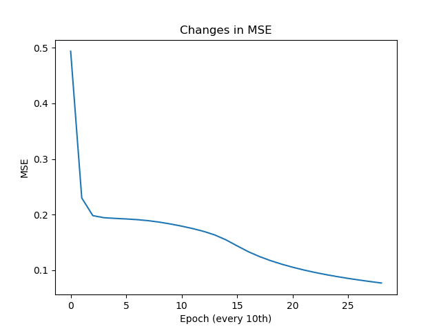
Changes in MSE
Our neural network can successfully do binary AND operations now!
Fun note
| A | B | Prediction |
|---|---|---|
| 2 | 0 | 1 |
| 0 | -1 | 0 |
| 45 | 203 | 1 |
| -21 | 0 | 0 |
| 0 | 85 | 1 |
| 0 | -328 | 0 |
Aside from being able to do binary AND operations, the neural network seems to always predict 1 when a positive number is used and 0 when a negative number is used.
Sadly, this remains a secret from us…
Conclusion
Implementing a neural network can be challenging at first, especially since a lot of articles makes it seem like its hard and you need to be a math genius to get it done. In reality, it’s fairly simple to do it. All you need to have is some basic knowledge in calculus and machine learning.
I hope this post helped you understand how a neural network functions and especially how it can be trained using the Backpropagation algorithm. If you have any suggestions, improvements, questions or whatever feel free to comment below!